classification(1) -- Alexnet、ZFNet、OverFeat
paper: ImageNet Classification with Deep Convolutional Neural Networks
We need large dataset to solve complex recognition tasks, and we need a model with a large learning capacity. Beside, model needs to have a generalization performance, not just perform well in a single dataset. Let’s start our CNN tour here.
Contributions
- large cnn used in the ILSVRC-2010 and ILSVRC-2012
- highly-optimized GPU implementation of 2D convolution and all the other operations inherent in training CNN
- features which improve CNN’s performance and reduce its training time
- techniques for preventing overfitting
Pre-proccessing
- image’s shorter side rescale to 256, then crop out the central 256x256 patch
- subtract the mean activity over the training set from each pixel
Architecture
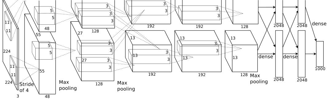
5 convolutional and 3 fc. LRN is used after the first and second convolutional layers.
### Features with the most important first
1. ReLU: make learning faster
2. Multi GPUs training
- one GPU’s(GTX 580) memory is not enough for training 1.2 million examples
- GPUs are able to read from and write to one another’s memory directly without going through host machine memory
- trains faster than one-GPU net and reduces top-1 and top-5 error rates by 1.7% and 1.2%
3. LRN(Local Response Normalization), while we do not use anymore, reduces top-1 and top-5 error rates by1.4% and 1.2%
4. overlapping pooling: use MaxPooling (kernel_size=3,stride=2), reduces top-1 and top-5 error rates by 0.4%and 0.3%
### Reducing Overfitting
1. Data augmentation
at train time, random crop 224x224 + horizontal reflections; at test time, crop 4 corner and 1 center patches (x5) and their horizontal reflections (x2), then average the predictions made by the network’s softmax layer on the ten patches. Fancy PCA, this scheme reduces the top-1 error rate by 1%
2. Dropout
### Training Details
1. optimizer: SGD with momentum=0.9 and weight decay=0.0005
2. initialize: a zero-mean Gaussian distribution with std=0.01, neuron biases in the second, fourth, fifth convolutional layers and fc layers with the constant 1
3. learning rate: use an equal learning rate for all layers, and divide the learning rate by 10 when validation error rate stops improving with the current lr
### Discussion
Depth really is important for achieving the results, the AlexNet’s performance degrades if a single convolutional layers is removed.
————————————–
paper: Visualizing and Understanding Convolutional Networks
Larger labeled training sets, powerful GPU, better regularization strategies achieved good performance in detection, such as AlexNet. We want to know how and why they work. Let’s look what happened in the network.
### Contributions
use a multi-layered deconvolutional network to visialize the input stimuli that excite individual feature maps at any layer in the model performs a sensitivity analysis of the classifier output by occluding portions of the input image, revealing which parts of the scene are important for classification.
* discuss the arcitecture of the network based on AlexNet.
### Architecture and Comparion with AlexNet
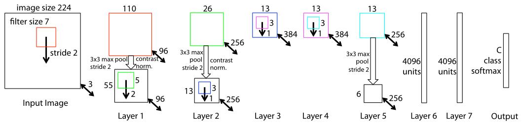
There are many similarities between ZFNet and AlexNet in Arcitecture and training details. Preprocessing, SGD optimizer, learning rate adjustment strategy, using dropout and so on, more details can be seen in AlexNet. While it initilize the network’s weight to 0.01 and bias to 0. And the structure is different in the first layer with different kernel size and stride for better visialization. This change silghtly outperforms the arcitecture of AlexNet. Layers 3,4,5 are replaced with dense connections not sparse connections in 2 GPUs.
Visualization with a deconvnet
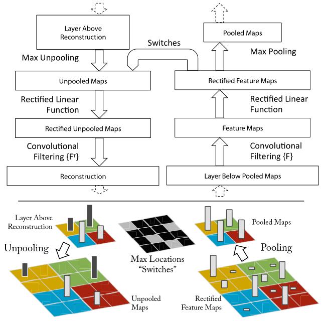
Here, deconvnets are not used in any learning capacity, just as a probe of an already trained connet.
Process: conv(learned filters) -> ReLU -> MaxPooling(need to save the location of the max value used in UnPooling) -> UnPooling -> ReLU -> deconv(use transposed versions of learned conv filters, this means flipping each filter vertically and horizontally.)
This and this explain the deconve processing very well. More things about convolution is A guide to convolution arithmetic for deep learning.
Something found in visialization(images can be seen in the paper)
- Feature Visialization: Layer 2 responds to corners and other edge/color conjunctions. Layer 3 has more complex invariances, capturing similar textures. Layer 4 shows significant variation, and is more class-specific: dog faces; bird’s legs. Layer 5 shows entire objects with significant pose variation.
- Feature Evolution during Training: The lower layers of the model can be seen to converge within a few epochs. However,
the upper layers only develop develop after a considerable number of epochs (40-50), demonstrating the need to let the models train until fully converged. - Occlusion Sensitivity: the model is localizing the objects within the scene, as the probability of the correct class drops significantly when the object is occluded. When occluder covers the image region that appears in the visualization, we see a strong drop in activity in the feature map.
Arcitecture Analysis
- Removing the fully connected layers (6,7) or two of the middle convolutional layers makes a relatively small difference to the error rate. However, removing both the middle convolution layers and the fully connected layers yields a model with only 4 layers whose performance is dramatically worse. This would suggest that the overall depth of the model is important for obtaining good performance.
- while making network fatter(increasing the size of middle conv layers and fc layers), it improves slightly and has the risk of overfitting.
- Using pre-trained model then fine tuning the softmax layer is much more better than model trained from beginning on the new set, shows the power of ImageNet feature extractor.
Discussion
- visualize what your network learned can be used to identify problems and so obtain better results.
- use models pre-trained in large datasets, such as ImageNet
paper: OverFeat: Integrated Recognition, Localization and Detection using Convolutional Networks
Classification, localization and detection are three computer vision tasks.The paper proposes a new integrated approach to these tasks with a singleConvNet.
Contributions
- use a single shared network to learn different tasks
- a feature extractor called OverFeat
Vision tasks from easy to hard
- classification: each image is assigned a single label corresponding to the main object in the image. Five guesses are allowed to find the correct answer.
- localization: compare to classification, a bounding box for the predicted object must be returned with each guess.
- detection: differs from localization in that there can be any number of objects in each image (including zero), and false positives are penalized by the mean average precision(mAP) measure.
Classification
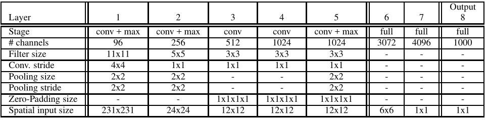
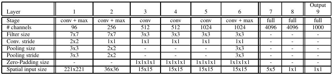
Two models are provided, a fast(top) and accurate(down) one. The accurate model is more accurate than the fast one, however it requires nearly twice as many connections.
This model is similar to AlexNet, but with the following differences: (i) no contrast normalization is used; (ii) pooling regions are non-overlapping; (iii) larger 1st and 2nd layer feature maps, thanks to a smaller stride (2 instead of 4).
For classification, we use accurate model. There are no special details in training, but using multi-scale for classification rather than averaging a fixed set of 10 views(4 cornersandcenter, with horizontal flip). Using the entire image by densely running the network at each location and at multiple scales yields more views for voting, which increases robustness while remaining efficient with convnets. The last fc layers are replaced by 1x1 convolution operations, The entire ConvNet is then simply a sequence of convolutions, max-pooling and thresholding operations exclusively. The main steps are as follows:
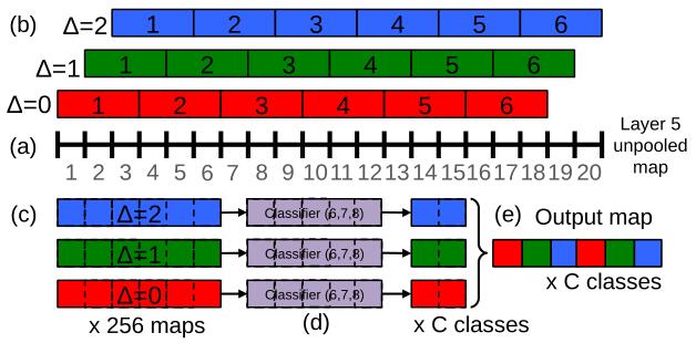
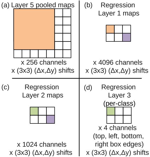
- As shown in the picture, suppose the size of unpooled layer 5 maps is 20x20x1024(1024 is number of channels);
- use 3x3 max pooling operation (non-overlapping regions), repeated 3x3 times for (∆x ,∆y) pixel offsets of {0,1,2}, then we get 3x3=9 maps with size 6x6x1024.
- The classifier can be seen as a box which has a fixed input size of 5x5 and produces a C-dimensional output vector for each location within the pooled maps. So 6x6 in and 2x2 out, we can get 3x3=9 maps with size 2x2xC.
- Then reshape the size to (2x3)x(2x3)xC=6x6xC, we get 36 outputs of classification.
- Then class-wise maxpooling, from 36xC to 1xC.
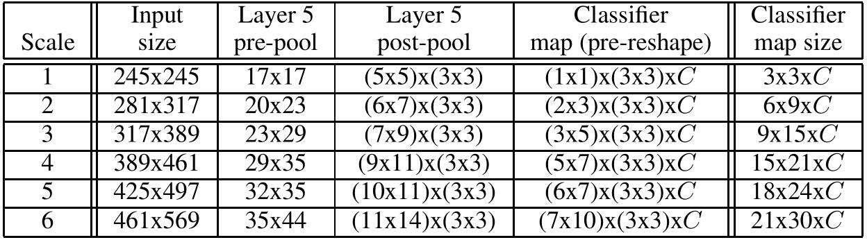
- Then average the resulting C-dimensional vectors from different scales and flips and take the top-1 or top-5 elements from the mean class vector. different scales are shown as follows:
Localization
Using classification-trained network and fixing the feature extraction layer(1-5), we add a regression network (just like classifier) and train it with L2 loss to predict object bounding boxes. We then combine the regression predictions with the classification results at each location.
The regression network outputs 4 units which specify the edges of the bounding box. And use the same (∆x ,∆y) pixel offsets operatin similar to classification. Besides, the final regressor layer is class-specific, having 1000 different versions, one for each class.
Then predict the set of classes in the top k for 6 scales, and conbine predictions using a greedy merge strategy (conbine boxed with high overlap ratio). The final predictionis given by taking the merged bounding boxes with maximum class scores.
Detection
Similar to classification training but need to predict background, Multiple location of an image may be trained simultaneously.